Procedural generation of organic shapes using Bézier curves
Table of Contents
Preface
A while ago I got an idea to create some «organic» shapes for 3D-printing. I learned a bunch of interesting stuff trying to do that. This post captures the essence of my experience.
The post starts with an introduction to the tools I am using. Then I present the concept of Bézier curves. I provide a bunch of illustrations to make it more intuitive and fun. After we are familiar with both the tools and the curves, I wrap up by showing how it works in practice.
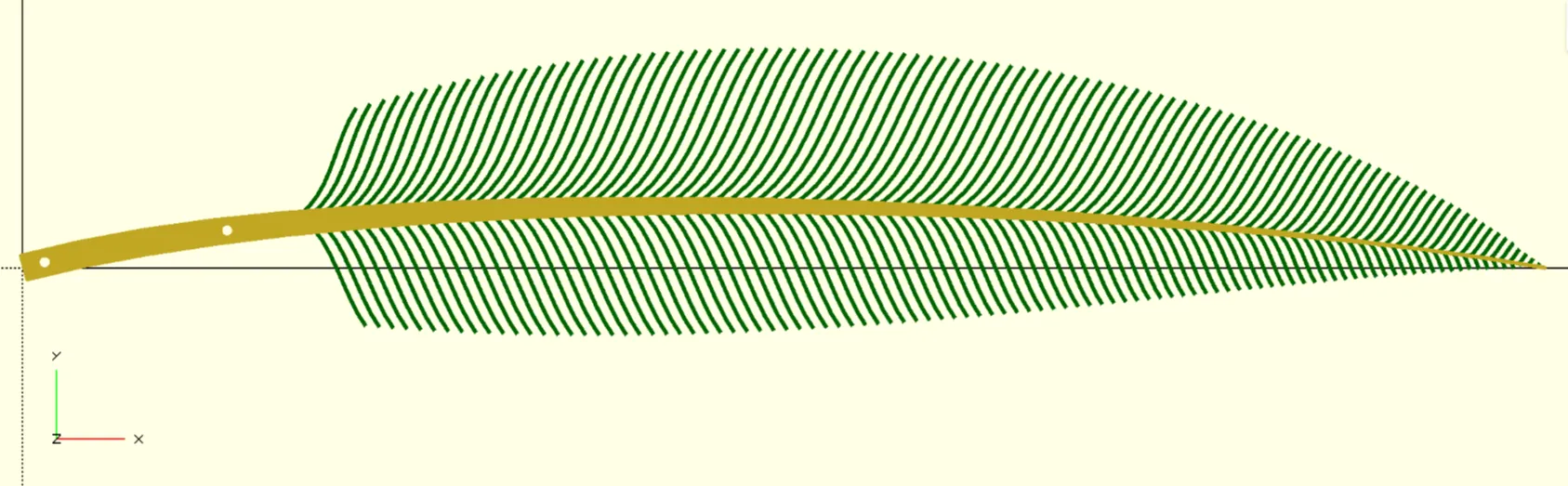
The resulting model to be 3D-printed
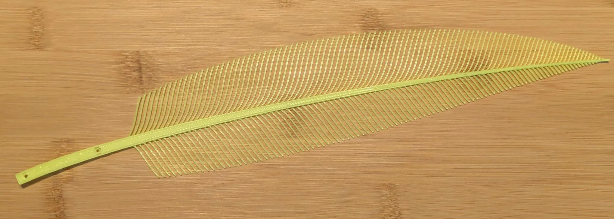
The result of 3D-printing said model
The post contains some maths, but understanding them should not be necessary for enjoying the content.
The tools
This project is something that I didn’t want to try and do using Autodesk Fusion, which I used for Hovert60 keyboard development. I also didn’t want to boot into Windows to use Fusion every time 😅
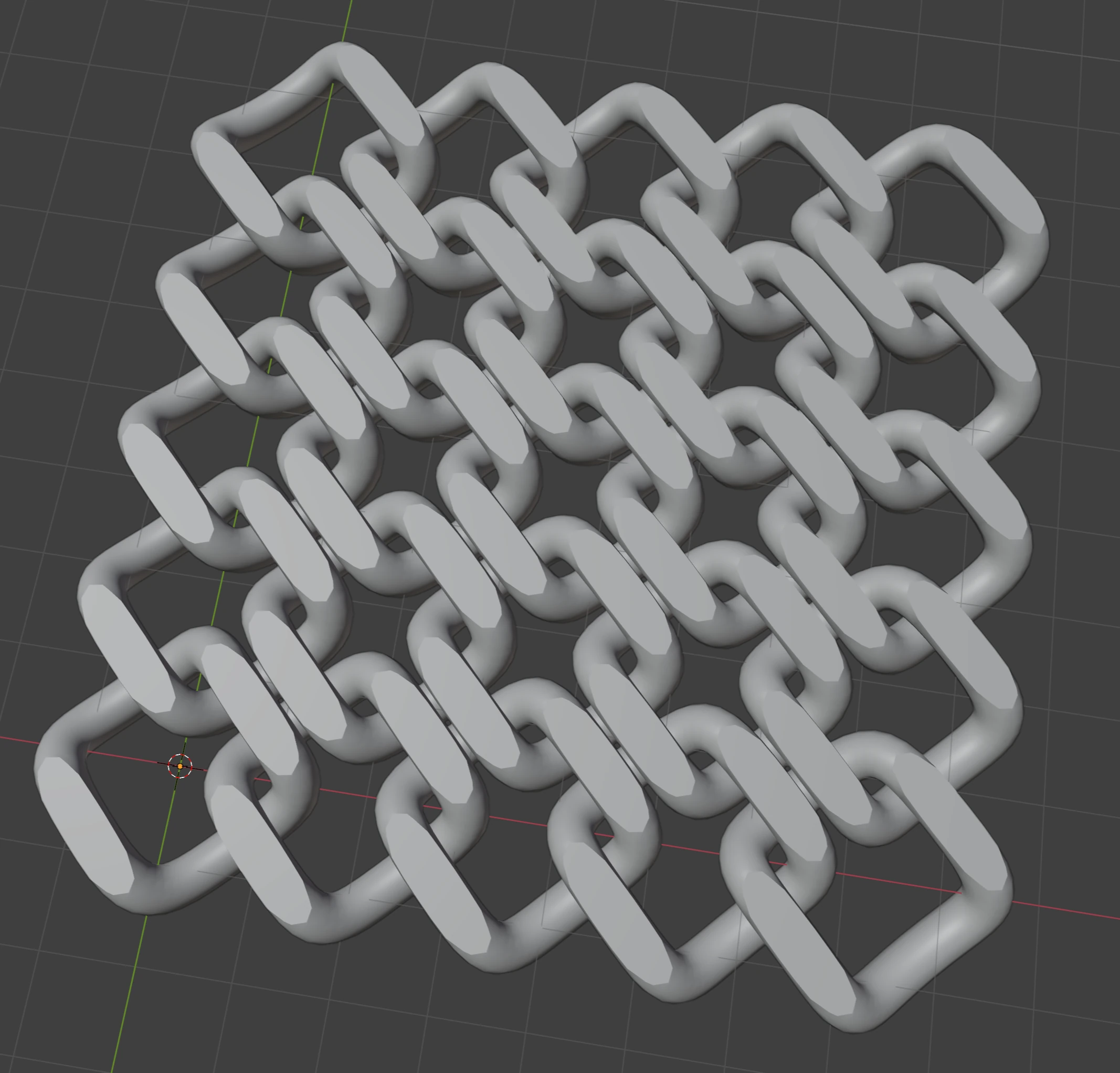
Print-in-place mail made in Blender using an Array Modifier applied to an expanded NURBS curve, and flattened with a Boolean Modifier for better bed adhesion
After some experiments with Blender and even with writing some custom G-code for 3D-printing, I stumbled upon a tool called OpenSCAD.
What is OpenSCAD?
OpenSCAD is a CAD program that allows modeling complex solid objects by combining simpler objects in various ways. Supported operations include:
- Creating primitive polygons like squares and other regular polygons (approximations of circles)
- Creating arbitrary polygons from a set of points
- Creating primitive polyhedra like cubes, prisms (approximations of cylinders), UV spheres
- Creating arbitraty polyhedra from a set of triangles
- Affine transformations of polygons and polyhedra
- Rotation
- Translation
- Scaling
- Mirroring
- Arbitrary transformations using a matrix
- Boolean operations on polygons and on polyhedra
- Union
- Intersection
- Difference
- Convex hull calculation for polygons and polyhedra
- Minkowski addition of polygons and polyhedra
- Offsetting a polygon’s outline
- Extrusion of 2D shapes into 3D shapes with linear or rotational movement
Unlike in many other tools, models in OpenSCAD are created by writing code rather than by interacting with a GUI. I think this approach unlocks several benefits.
For instance, my existing software development skills translate to OpenSCAD nicely, as it allows storing the code for my models in Git and provides capabilities for code reuse. It removes the need to learn a complex set of keyboard shortcuts and menu items, instead providing a simple API for which it has a cheatsheet.
But OpenSCAD also has a bunch of drawbacks compared to other CAD software. It does not use the concept of constraints, and the user has to figure out the formulas even for simple things. The simplicity of the API I mentioned requires a high degree of creativity from the user when making advanced designs. As a result, creating complex models can get overwhelming.
In their work, software developers can spend some extra effort on making their code more «future-proof». The code could be organised more neatly, variables and functions could be named appropriately and so on. When working with OpenSCAD, you end up having to do the same. But organizing code and thinking of right names for parts of your designs can be quite hard.
I think these limitations of OpenSCAD pose an interesting challenge for its users. I can’t say if they make OpenSCAD less suited for professional work, but they definitely can make it more enjoyable.
Bézier curves
When I started, I didn’t know what I want to achieve, but I knew I wanted to use Bézier curves for this small project.
You might have encountered these curves in programs like Inkscape or Adobe Illustrator.
There are 3 ways to use them in OpenSCAD:
- Through a 3rd-party library (which is boring)
- Imprort an SVG (which is not flexible, and also boring)
- Implement the curves by myself (yeah, try to guess where this is going…)
To implement the curves, I needed to revisit some theory, which I will explain here. Feel free to skip the maths – I think the pictures with their flavour text should be enough to get the basic idea.
The Basics
Before we can talk talk about advanced stuff, I should make sure we are on the same page with regards to the basics. I will be very brief. There are two very simple concepts that serve as a foundation for Bézier curves. They are:
- Vectors and operations on them
- Linear interpolation between two vectors
In this post, we are working on a Cartesian plane. That implies:
- There are 2 axes (X-axis and Y-axis), 2 dimensions
- The axes are perpendicular to each other
- Any point (or vector) on the plane can be defined using a pair of two real numbers
You might have learned about vectors in school. For this post, what matters is:
- A vector is a pair of two real numbers
- Two vectors can be added together
- Two vectors can be subtracted from each other
- A vector can be multiplied by a scalar (a real number)
- Each vector has some length

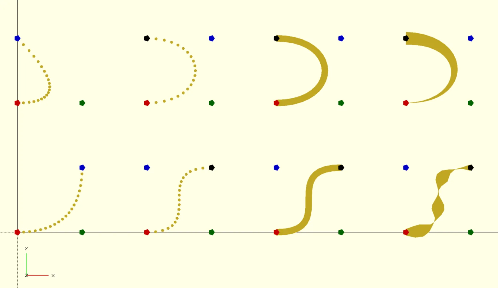
Examples of operations on vectors. Left: two vectors. Middle-Top: difference of two vectors. Middle-Bottom: multiplying vectors by scalars. Right-Top: sum of two vectors. Right-Bottom: length of a vector.
Let’s look at the examples. Given two vectors and ,
Their sum is:
Their difference is:
Multiplying them by a scalar:
For a different vector ,
It’s length can be calculated by the Pythagorean theorem:
Now, the remaining piece of the puzzle is a function called which stands for Linear interpolation. This function receives 3 values: 2 values and to interpolate between, and a parameter . and can be real numbers, but they can also be vectors (with the same dimensionality).
can be defined like this:
Note the values of the function for at the ends of the interval:
Now, if we calculate for all for some fixed and , we get a set of points that live on the line segment connecting and .

Quadratic Bézier curves


Cubic Bézier curves


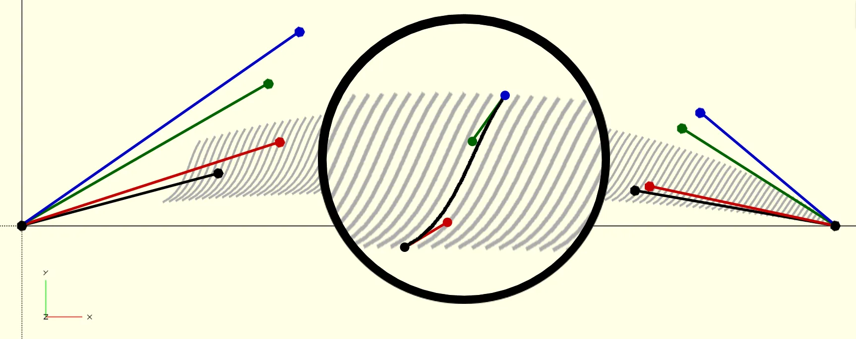
Derivative of a Bézier curve

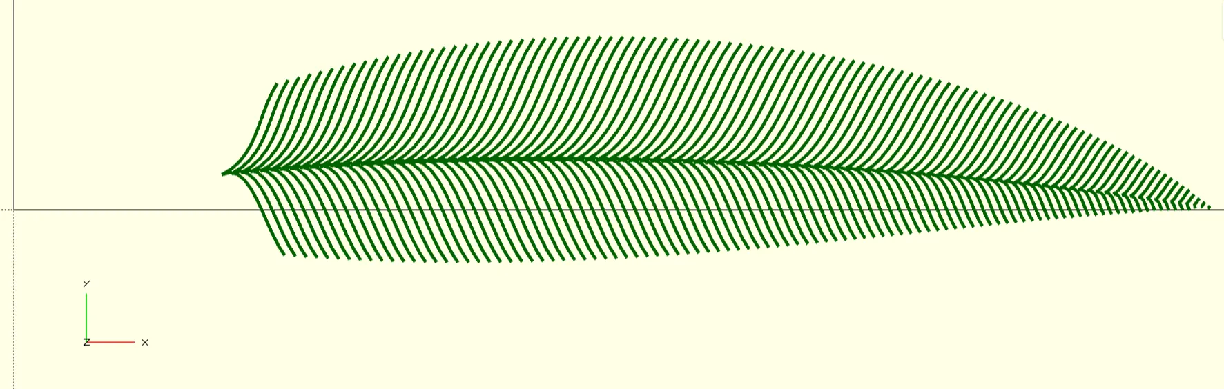
Stroke expansion


Putting it all together
Results
…