In search of the Visibility Polygon
Table of Contents
I have been building a 2D game for fun recently. Once I implemented a basic lighting system for it, I understood that I want game objects to cast shadows. There are multiple ways to achieve that, and the approach I selected is based on visibility polygons.
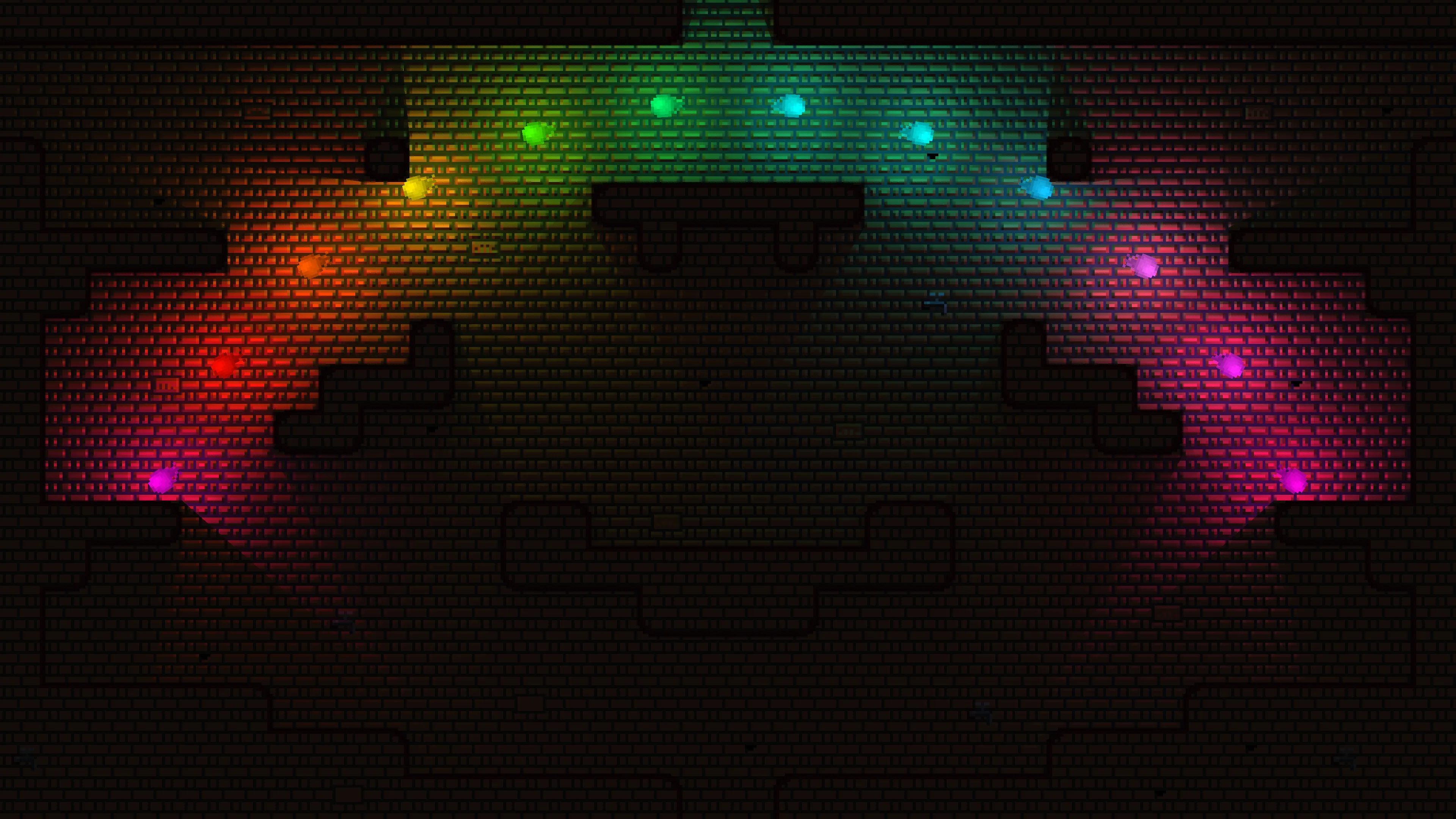
Fig. 1. A frame from the game I am building, with differently colored flames lighting up different areas based on their visibility
A visibility polygon represents the area that, for a given arrangement of occluding objects, has a direct line of sight to a certain point (called the query point). You can read more about them here:
- Visibility polygon on Wikipedia
- 2D Visibility on Red Blob Games
I find the problem of calculating the visibility polygon interesting, and in this post I will tell you how I implemented an algorithm that finds them. I think the algorithm itself and the optimisations involved are conceptually cool, so I am excited to illustrate and describe them.

Fig. 2. This is what a visibility polygon looks like. The occluding objects are purple, the polygon is yellow, and the query point is red.
The algorithm I implemented is based on a description I found in 1 under the section «3.2 Algorithm of Asano». That paper actually suggests a different algorithm for this problem, but I found the algorithm of Asano more fun. That paper also references a source for the algorithm 2 , but I found the short description more interesting to work with. Also, 2 is quite hard to access.
In this post I will describe the implementation of that algorithm. There are some basic concepts I expect the reader to be familiar with, I will cover them briefly. There will also be some additional ideas that I will explain in more detail further in the post.
Basic concepts
There are some common symbols I am going to use:
| Symbol | Meaning |
|---|---|
| for all … | |
| there exists such that … | |
| and (are true) | |
| or (or both) (are true) | |
| implies | |
| if and only if | |
| is defined as |
A set is a collection of objects, which are called elements of the set. The order of the elements in the set does not matter.
Sets can be declared by specifying the rules of element inclusion. For a condition and expression , a set of all values of for which is true can be denoted like this:
For example, the set of all integers
The following are some symbols related to sets:
| Symbol | Meaning |
|---|---|
| is an element of set | |
| is a subset of | |
| intersection of sets and |
The set of all real numbers 3 is denoted as .
The set of all pairs of real numbers
- A point is represented using an element of 4.
- A vector is also represented using an element of , even though it has a different meaning 5.
- A line is a set of points that is infinitely long and has no width 6. A line can be defined by two distinct points.
- A segment is an uninterrupted subset of a line 7. A segment can be defined by two distinct points. All segments in this post are closed segments, which means they include their endpoints.
In this post, I use the following notation:
A point is collinear 8 with a segment if it lies on the line defined by that segment’s endpoints.
A pair of segments is collinear 8 if all of their points are on the same line.
An intersection of two lines 9 can be one of:
- An empty set (then the two lines are parallel),
- A single point,
- A line (then the lines are equal).
An intersection of two segments 10 can be one of:
- An empty set (no intersection, the segments may still be parallel and collinear),
- A single point,
- A segment (then the segments are collinear, but may not be equal).
Algorithm inputs and outputs
The algorithm needs the following inputs:
- a query point ,
- a set of segments .
No segment in should include .
No two distinct segments in are allowed to intersect, unless their intersection is a single point that is an endpoint of both of those segments.
Running the algorithm produces a set of segments that represents the surfaces visible from . Each segment in is a subset of some segment from .
From , the actual polygon can be obtained by combining the endpoints of each of the segments in with to form triangles. The polygon is the union of all such triangles
The outline of the polygon can also be trivially generated with a slight modification to the algorithm, which is left as an exercise for the reader.
Algorithm overview
To calculate the visibility polygon, we will «visit» all of the segment endpoints, keeping track of which segment is the nearest to at all times.
This is a sweep line algorithm 11. The sweep line in this case is the line that connects with the current endpoint. As the current endpoint changes, the line rotates around .
Let be the number of segments in the input.
This problem can be solved naively in time. For example:
- Sort segment endpoints by their position relative to .
- For each endpoint , find all intersections between and all other segments. Use that information to keep track of which segment is the nearest to .
- Whenever the segment nearest to changes, register that, and build up the visibility polygon out of the relevant subsegments.
An optimisation allows us to cut down the time to . Instead of keeping track of just the nearest segment, we will keep track of all segments that are currently intersected by our sweep line (henceforth called active segments).
As the sweep line goes through segment endpoints, we will be «activating» and «deactivating» corresponding segments. In practice, given some endpoint, it can be difficult to tell what to do with it on the fly. For this reason, all endpoints are designated as or events. See Ordering endpoints within a segment.
To keep track of currently active segments, an ordered set can be used. Common implementations of ordered sets 12 can do insertion and removal in time – that’s exactly what we need!
Note, though, that we need to define the ordering between the segments to store them in an ordered set. It’s a bit tricky to do, so see Ordering segments by distance to a point.
Summary
Time to bring this all together. This is what the algorithm does:
- Prepare the input data:
- Create a set of all segment endpoints, keeping track of which segment they came from;
- For each of the endpoints, designate it is a or an event;
- Order the endpoints based on the direction from to the endpoint.
- Determine the initial state – choose the first endpoint and find all segments that are active when the sweep line passes through it.
- Go over all events, doing the following:
- Activate the segment if this is a event,
- Deactivate the segment if this is an event,
- Save a new visibility segment whenever the segment closest to changes.
Let’s go through an example, and then we can look into the fun implementation detais.
Example
In this example, we will …
Example: defining input data
Let’s define some example input data. The input data consists of the point and a set of segments . You can see the input configuration in Fig. 3.1. It contains the point (the star in the middle) and 16 segments (purple lines) connecting 16 points.
Note the 4 segments that together form a rectangle that surrounds everything else. This guarantees that there is at least one segment in any direction from , as explained in the Side note: Implications on the output.

Fig. 3.1. Example input data.
For simplicity, let’s say that . Let’s also choose coordinates for all of the points:
And, based on those points, let’s define the set of occluding segments
Example: ordering segment endpoints
Now that we defined the input data, we need to order all segment endpoints by their position relative to . For each point , we will use the angle between the and the -axis shown in Fig. 3.2.

Fig. 3.2. Ordering points based on the angle between the -axis (in blue) and a vector from to that point.
We also need to keep track of what segment each endpoint came from, and designate the endpoints as or of that segment. Read more about how this is done in the Ordering endpoints section.
The result of this step is an ordered list of all endpoints, together with their / designation and their segment:
- in is ,
- in is ,
- in is ,
- in is ,
- in is ,
- in is ,
- in is ,
- in is ,
- in is ,
- in is ,
- in is ,
- in is ,
- in is ,
- in is ,
- in is ,
- in is ,
- in is ,
- in is ,
- in is ,
- in is ,
- in is ,
- in is ,
- in is ,
- in is ,
- in is ,
- in is ,
- in is ,
- in is ,
- in is ,
- in is ,
- in is ,
- in is .
Example: finding the initial state
Our sweep line will start from the first point in the list. As you might have noticed in Fig. 3.2, the positive direction of the -axis intersects with some of the segments. We need to determine which segments are initially intersected before we can start the main sweep.
To do that, we will perform an «initialisation» sweep, in which we will simply track segment and events. Let’s say we have a (mutable) set of active segmens which starts empty. Then, let’s go through the ordered list of all endpoints and:
- if the endpoint is a of a segment, add the segment to the set,
- if it is an of a segment that is present in the set, remove the segment from the set,
- otherwise, keep the set intact.
After that, will contain the segments that have «started» but have not yet «ended».
Example: sweeping the line
Fig. 3.3 shows the lines connecting with all of the segment endpoints. It also shows points , , , and that represent projections of the corresponding points onto the next closest segment in that direction.

Fig. 3.3. Segments connecting with all other points.
Example: result

Fig. 3.4.
Implementation details
Ordering endpoints
- by angle
For each point , let’s find the angle makes with the -axis. It can be calculated using the function
- within a segment

Fig. 4.1, 4.2, 4.3.
Determining whether a point lies in a half-plane
A naive implementation of can …

Fig. 5.
…
Ordering segments by distance to a point
The algorithm features a segment comparison routine that is aimed at decreasing the cost of performing the comparison by reducing the number of required floating point operations.
The cheap segment comparison routine is only valid under the following assumptions:
- Any two segments can only be compared between each other if a line can be drawn that includes the query point and a point from each of the segments
- The segments do not intersect between each other with the exception of intersections that yield their endpoints
The comparison routine can be simplified if all segments collinear with the query point are removed from the input data. For completeness, cases when the query point is collinear with the segments are still considered below.
Both segments are collinear with the query point

Fig. 6.1, 6.2.
One of the segments is collinear with the query point

Fig. 6.3, 6.4.

Fig. 6.5, 6.6.

Fig. 6.7, 6.8.
None of the segments are collinear with the query point

Fig. 6.9, 6.10.

Fig. 6.11, 6.12.

Fig. 6.13, 6.14. 6.15.

Fig. 6.16, 6.17.

Fig. 6.18, 6.19.
Reducing input size
…
Francisc Bungiu, Michael Hemmer, John Hershberger, Kan Huang, Alexander Kröller (2014). Efficient Computation of Visibility Polygons. ↩︎
Asano, Tetsuo (1985). An efficient algorithm for finding the visibility polygon for a polygonal region with holes. Institute of Electronics, Information, and Communication Engineers. Vol. 68. pp. 557–559. ↩︎ ↩︎
Real number on Wikipedia ↩︎
Euclidean plane on Wikipedia ↩︎
Euclidean vector on Wikipedia ↩︎
Line segment on Wikipedia ↩︎
Collinearity on Wikipedia ↩︎ ↩︎
Line–line intersection on Wikipedia ↩︎
Intersection of two line segments on Wikipedia ↩︎
Sweep line algorithm on Wikipedia. ↩︎
For example, BTreeSet in Rust. Read about BTrees on Wikipedia. ↩︎